Simulate, Analyse, Plot ...

AIM : Let say the aim is to prepare a movie of coarse grained description of the system. In this example the 2-dimensionl lattice has been divided into several sub-square lattices. Then depending on the order parameter values (average) in the sub-square lattices, the color has been chosen and finally each frame has been added using 'addframe'. clear all; close all; aviobj = avifile('box_movie.avi','compression','None'); aviobj.KeyFramePerSec = 1; fig = figure; fid = fopen('fort.214'); nbox = 25; nframes = 9900; for i = 1:1:nframes     A = fscanf(fid, '%g', [1 nbox]);     if (i < 3500) && (mod(i,5) == 0)     % Draw smaller boxes         xstart = 0;     ystart = 0;     xlen = 1;     ylen = 1;         rectangle('position', [xstart, ystart, xlen, ylen]);     nx = floor(sqrt(nbox));     ny = nx;     dx = xlen/(nx);     dy = ylen/(ny);     count = 0;     for i = 1:nx         x = xstart + (i-1)*dx;         for j = 1:ny    

2D movie of different types of particles, using 'gscatter' and 'addframe': MATLAB Let say, the goal is to create a movie file from different snapshots and the available raw data has the co-ordinates and corresponding order parameters value. By the following way one will end up with a 2D video of (x,y) data having different types of particles characterized by 'z' values. The two key commands used are gscatter and addframe . In this example all the particles are of two types, so I used two types of color function (blue and red) to distinguish them. Finally, I was looking to fill up the markers, however I could not find any suitable way to fill them (If anybody knows about it please let me know). Instead of searching for filling the markers I used a crude way of increasing linewidth of the markers, which eventually ended up, what I needed :).   %To create movie from scatter plot aviobj = avifile('movie.avi','compression','None'); fig=fi

Playing with shell Here I have summarized few shell script which I routinely use. All the informations are floating in the net. It needs just a little bit of careful google search and then test by yourself. Start with a simple one: Addition, subtraction, multiplication and division  Let say a=10, b=5, c=a+b or a-b or a/b or a*b. How to do that using Bash (Born Again Shell) shell scripting? However, bash script will give result in integer number.    a=10 b=5 c=$(($a+$b)) echo $c It will print 15. c=$(($a-$b)) echo $c It will print 5. c=$(($a/$b)) echo $c It will print 2.   c=$(($a*$b)) echo $c It will print 50. Let say you would like to do little complex calculation like  c=(a+b)/a*10 - b/(a-100)   c=$(($(($a+$b))/$(($a*10))-$(($b/$(($a-100)))))) What if one needs to get the same operation for real numbers? One needs to use then awk script. a=10.5 b=2.5 c=$(echo $a $b | awk '{ print $1 + $2 }') echo

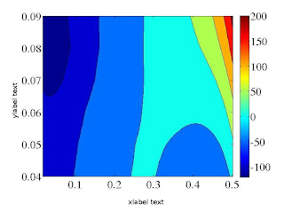
2D CONTOUR PLOT IN MATLAB %This .m file will generate 2D contour plot clear all; close all; L1 = load('dataset1.dat'); % [Let say the data set has 220 X co-ordinate data, and 6 Y co-ordinate data, and for these X and Y coordinate combinations Z coordinate values are there. Now, one has to form a matrix to get contour plot which will be generated in the following way] N1=6;      N2=220; k = 1; for i = 1 : 1 : N1   for j = 1 : 1: N2      k = (i - 1) * N2 + j;     X1(j,i)  = L1(k, 1);     Y1(j,i)  = L1(k, 2);     Z1(j,i)  = L1(k, 3);   end  end  contourf(X1, Y1, Z1); lighting gouraud xlim([0.0 0.6]) ylim([0.04 0.09]) set(gca, 'xtick', 0.0:0.1:0.6,'Fontsize', 15) set(gca, 'ytick', 0.04:0.01:0.09,'Fontsize', 15) xlabel('xlabel text','Fontsize', 20); ylabel('ylabel text','FontSize', 20);

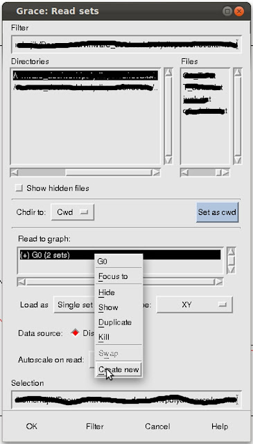
Grace is an opensource data-analysis/plotting software. Grace runs on practically any version of Unix-like OS. As well, it has been successfully ported to Win9*/NT/2000/XP (some minor functionality may be missing, though). The inset plot can be generated by following way: Give command in terminal: xmgrace dataset1.dat , (or import data by Data -> Import -> ASCII in other platforms) will create the plot of dataset1.dat in the main window (call it Graph1). Now for creating inset of another dataset let say dataset2.dat in the same graph please follow the following steps. Data -> Import -> ASCII to open the " Grace:Read Sets " dialogue box.  Graph 1 created in step 1 , is labelled G0 . In the " Read to Graph " section the " (+) G0 " graph is selected by default.  Right-click on the " (+) G0 " to open the pop-up menu (see the image).  Select " Create new ". It will create ' (+) G1 ' empty graph. 

Few basic commands: After successful installation you are ready to go with GROMACS. A basic tutorial for simulating Lysozyme in water can be found here . Here, I will compile few necessary commands in one page. Execute .pdb file to generate initial .gro file pdb2gmx -f initial.pdb -o processed.gro If you do not have topology file of your molecule, you can generate one by using g_x2top -f file.gro -o topol.top -ff select -name ABC -noparam -pbc   In the above command line 'ABC ' is your molecule NAME, e.g. if you are simulating carbon nanotube and you are calling carbon nanotube as CNT, then ABC = CNT Define your simulation box using editconf: editconf -f processed.gro -o newbox.gro -c -d 1.0 -bt cubic Solvation of defined box genbox -cp newbox.gro -cs spc216.gro -o newbox_solv.gro -p topol.top Include ions if necessary: grompp -f ions.mdp -c newbox_solv.gro -p topol.top -o ions.tpr genion -s ions.tpr -o newbox_solv_ions.gro -p topol.top -pname NA -